Background
While going through the literatures, I came across two landmark articles on the evolution of Monoclonal Gammopathy of Unknown Significance (MGUS) and Smoldering Multiple Myeloma (SMM) by the Mayo Clinic Group headed by Dr Robert Kyle. These articles described the evolution of MGUS and SMM into symptomatic myeloma by reporting cumulative proportion of developing symptomatic myeloma in a population based follow up study.
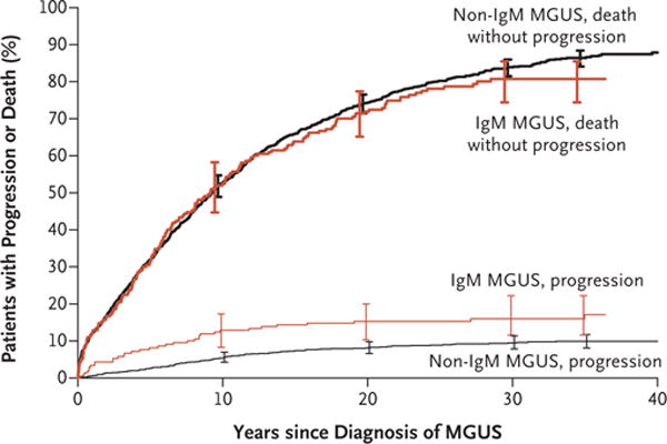
The following figure depicts the progression of MGUS into symptomatic myeloma
And the following figure depicts the progression of SMM into symptomatic myeloma

By looking at the above figures, I wanted to ascertain the behavior of early stage plasma cell dyscrasia (PCD) patients with respect to their hazard to develop symptomatic myeloma.
Loading libraries and functions
import numpy as np
import scipy.stats as st
import matplotlib.pyplot as plt
import lifelines as ll
%matplotlib inline
fsize = (10, 6)
kmf = ll.KaplanMeierFitter()
ajf = ll.AalenJohansenFitter()
def truncate(t0, t1, times, events):
    times_mod = []
    events_mod = []

    for t, e in zip(times, events):
        if t >= t0 and t < t1:
            times_mod.append(t - t0)
            events_mod.append(e)
        elif t >= t0 and t >= t1:
            times_mod.append(t1 - t0)
            events_mod.append(0)
    return (times_mod, events_mod)
def tlines_severity (sev0, times, trunc_time):
    res_times = []
    for t in times:
        tsev0 = t * sev0 / 100
        if tsev0 < trunc_time:
            res_times.append(t)
    res_times = np.array(res_times)
    trunc_times = np.clip(res_times, a_min = None, a_max = trunc_time) - (res_times * sev0 / 100)
    trunc_events = np.ones(len(trunc_times))
    trunc_events = np.where(res_times > trunc_time, 2, 1)

    return (list(trunc_times), list(trunc_events))
def hazards_severity(sev0, l_times, hrs, trunc_time):
    ns = []
    res = {}
    N = 0
    for h, times in zip(hrs, l_times):
        ctr = 0
        for t in times:
            tsev0 = t * sev0 / 100
            if tsev0 < trunc_time:
                ctr += 1
                N += 1
        ns.append(ctr)
    for h, n in zip(hrs, ns):
        res[h] = n / N
    return res
Model 1: Patient with increasing hazard
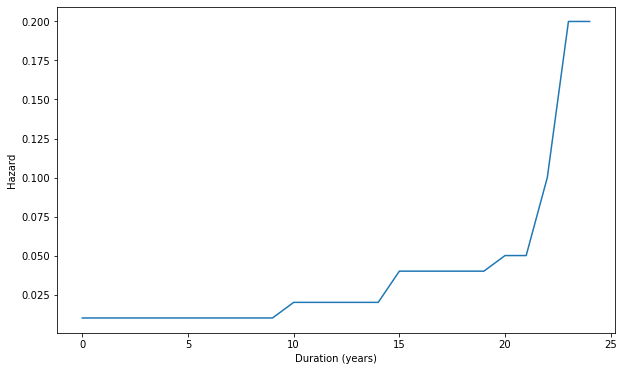
The hypothesis for this model is that the disease starts from 1 cell stage and then there is progressive increasing hazard to develop myeloma with passing time along with increasing severity. The hazard increases as the disease progresses in a say non linear fashion. We catch patients at different times in their history.
We make a vector with increasing hazard as follows
hr = [100] * 10 + [50] * 5 + [25] * 5 + [20, 20, 10, 5, 5]
f, ax = plt.subplots(figsize = fsize)
ax.plot([1/h for h in hr])
ax.set_xlabel('Duration (years)')
_ = ax.set_ylabel('Hazard')
Running simulation
We will run simulation with 1000 patients, with 25 years of follow up and the hazard as depicted in the graph above. The steps in simulation in depicted as below
times = []
events = []
n_sim = 1000

for n in range(n_sim):
    for t, h in enumerate(hr):
        t_event = np.random.exponential(h)
        if t_event <= 1:
            times.append(t + t_event)
            events.append(1)
        else:
            if t == len(hr) - 1:
                times.append(t + 1)
                events.append(0)
f, ax = plt.subplots(figsize = fsize)
kmf.fit(times, events).plot_cumulative_density(ax = ax)
ax.set_xlabel("Duration (years)")
_ = ax.set_ylabel("Cumulative proportion")
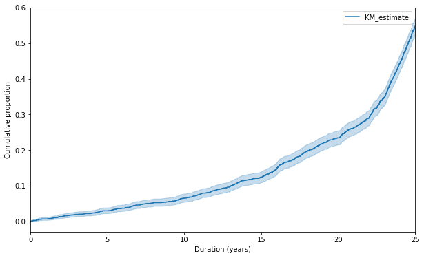
The above plot shows the cumulative proportion of progressing into symptomatic myeloma. We can see that rate of progression into myeloma increases at the time goes by, which is not the way MGUS and SMM behave in real life situation, where cumulative proportion plateaus off after certain duration.
Plateauing off of the cumulative proportion curve suggests either constant hazard or decreasing hazard disease process. And in the present hypothesis, the hazard increases with time.
Cumulative probability curves stratified with increasing duration of illness
Cumulative probability of progression should increase with increasing duration of illness, as is evident from both the trials. Let us divide the time points of diagnosing a patient into 1 years (equivalent of MGUS), 10 years (late MGUS) and 15 years (equivalent of SMM) post initiation of the disease and observe the cumulative probability of disease progression with starting time being the time of detection of the disease.
f, ax = plt.subplots(figsize = fsize)
for t0, t1 in [(1, 25), (10, 25), (15, 25)]:
    t_int, e_int = truncate(t0, t1, times, events)
    kmf.fit(t_int, e_int).plot_cumulative_density(ax = ax, label = '{} years'.format(t0))
ax.set_xlim(0, 10)
ax.set_xlabel('Duration (years)')
_ = ax.set_ylabel('Cumulative probability of progression')
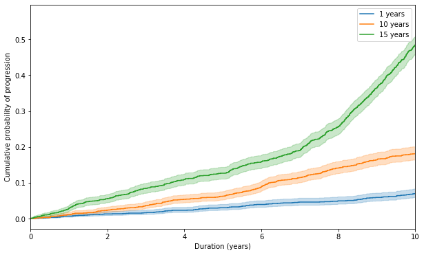
As we can see that although the cumulative probability of disease progression increases with disease duration, but the shape of the curves are concave downwards, which indicates the increasing hazard with disease duration, especially in group with late disease detection, which is not matching with the real life data.
We conclude that the present model of time varying hazard which is same all the patients does not hold good.
Model 2: Patients with different hazards
We now consider another hypothesis which states that
The hazard of disease progression is constant with respect to time and disease severity for each patient (can be modelled as exponential distribution).
The hazard of disease progression is different for each patient. Some patients have indolent, slowly progressing disease and some patients have aggressive, rapidly progressing disease.
The population is a mixture of patients with different hazards.
Running simulation
We will run simulation with hazard rate of 0.01, 0.05, 0.1 and 0.2 for 100 patients each.
f, ax = plt.subplots(figsize = (10, 6))
l_times = []
hrs = [100, 20, 10, 5]
n_pat = [100, 100, 100, 100]
for h, n in zip(hrs, n_pat):
    ts = list(np.random.exponential(h, n))
    l_times.append(ts)
    kmf.fit(ts, np.ones(len(ts))).plot_cumulative_density(ax = ax, label = h)
times = [j for i in l_times for j in i]
events = list(np.ones(len(times)))
kmf.fit(times, events).plot_cumulative_density(ax = ax, label = 'Total')
_ = ax.set_xlim(0, 20)
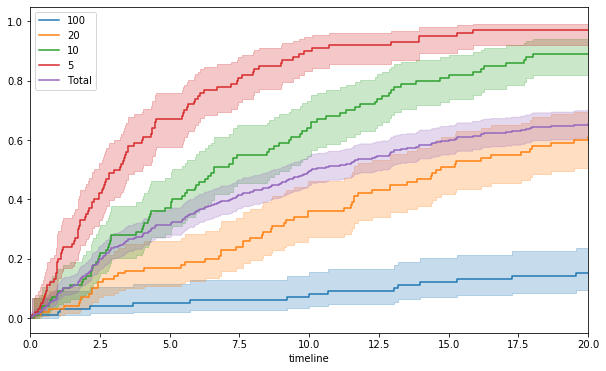
The above curves show predictably that patients with more aggressive disease have higher cumulative probability of progressing to symptomatic myeloma, and the shape of curves are matching with those seen in the trials.
Understanding severity of disease (disease load)
There are two different concepts in disease like PCD:
Disease severity (disease load): The disease load means the amount of disease that is present in a patient at a particular time point. Depending on the disease load, patient can be classified as having MGUS, SMM or overt MM. We hypothesise that disease load of every patient will increase with time at different rates.
Rate of disease progression: The rate of disease progression is the speed at which the disease load is increasing. Patients with aggressive disease will have higher rate of disease progression, whereas indolent disease will have lower rate of disease progression. The hazard rate depicts the rate of disease progression.
Every patient of PCD will traverse through all the severity of the disease, albeit at different rates, which means that every patient will go through the stages of MGUS and SMM. Patients with aggressive disease will stay in each stage for shorter duration time, before progressing into symptomatic myeloma and patients with indolent disease will remain in each stage for a longer duration before progressing.
Our goal in treating patients with PCD is to identify patients with aggressive disease and tackle them aggressively and leave the patients with indolent disease as it is.
It may happen that a significant number of patients having indolent disease will die of some other cause before progressing to myeloma.
If we select patients with increased disease load (which is what we do in trials), we will get more number of patients who have aggressive disease than if we select patients with indolent disease. There is a selection bias in the whole process. If we select a patient with increased disease load, there is more chance that that patient will have aggressive disease.
It is also true, that time to progression will be smaller in patients with increase disease load than the patient with same hazard with lower disease load, as the patient will have traverse more duration to reach the stage of increased disease load than to reach the stage of lower disease load, which means that the time to reach overt myeloma is shorter in former case.
Distribution of patients with different hazards with different severity
We define severity as a numeric with range from 0 to 100 (means highest disease severity), which will increase linearly with time duration after onset of the disease.
import pandas as pd
res = []
sevs = [10, 20, 50, 80, 90]
for sev in sevs:
    res.append(hazards_severity(sev, l_times, hrs, 20))
pd.DataFrame(res, index = sevs).round(decimals = 4)
| 100 | 20 | 10 | 5 | |
|---|---|---|---|---|
| 10 | 0.2228 | 0.2591 | 0.2591 | 0.2591 |
| 20 | 0.1694 | 0.2750 | 0.2778 | 0.2778 |
| 50 | 0.1094 | 0.2688 | 0.3094 | 0.3125 |
| 80 | 0.0786 | 0.2393 | 0.3286 | 0.3536 |
| 90 | 0.0733 | 0.2344 | 0.3333 | 0.3590 |
In the above table, we can see that with increasing severity (as depicted by the rows, 10, 20, …, 90), the proportion of patients who have aggressive disease (depicted by column labelled 5) increases and proportion of patients who have indolent disease (depicted by column labelled 100). We have truncated the time duration to 20 years from origin of disease, at which time we assume that all patients die.
Cumulative incidence of progression stratified with severity of disease at diagnosis
f, ax = plt.subplots(figsize = (10, 6))
for sev in sevs:
    t, e = tlines_severity(sev, times, 20)
    ajf.fit(t, e, 1).plot(ax = ax, label = 'severity: {}'.format(sev))
ax.set_xlabel('Duration (years)')
ax.set_ylabel('Cumulative Incidence of progression (death as competing risk)')
_ = ax.set_xlim(0, 10)
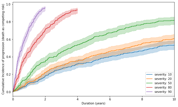
The above graph clearly depicts that with increasing severity, the cumulative incidence of progression increases with shape of curves being concave downwards, as is in real life trial data.
Conclusion
Model 2 and its hypotheses seems to be valid in real life situation, which has got a significant impact on the way we think about PCD and its treatment.